Data Assimilation
1. Data Assimilation
The main problem that is considered is how to correct our understanding of measurements done in the presence of noise. Given certain quantities like a measurement from a sensor, a distribution from which the process generates data, or new measurements after the first, we ask ourselves, how can we combine all given information into a calculation.
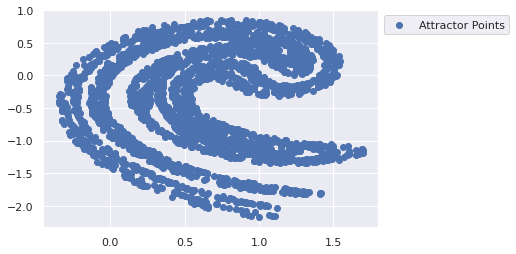
2. Ikeda Map Example
In this example, we consider the Ikeda map. It is a discrete dynamical system governed by:
\begin{align} x_{n + 1} &= 1 + u (x_{n} \cos(t_{n}) - y_{n} \sin(t_{n})) \\ y_{n + 1} &= u(x_{n} \sin(t_{n}) + y_{n} \cos(t_{n})) \end{align}Where \( u \) is some parameter and
\[ t_{n} = 0.4 - \frac{6}{1 + x_{n}^{2} + y_{n}^{2}} \]
2.1. Preamble
import jax
import flax

import jax.numpy as jnp
from jax import jit
from jax import lax

import matplotlib.pyplot as plt
import seaborn as sns
sns.set()

key = jax.random.key(0)
key, subkey = jax.random.split(key)
2.2. Implementation
We can implement this very easily in JAX or TensorFlow. For now I will be using JAX as I have a bit of a crush on the software at the moment.
@jit
def ikeda_update(point):
    u = 0.9
    x, y = point[...,0], point[...,1]
    t = 0.4 - (6 / (1 + x ** 2 + y ** 2))
    x_new = 1 + u * (x * jnp.cos(t) - y * jnp.sin(t))
    y_new = u * (x * jnp.sin(t) + y * jnp.cos(t))
    return jnp.stack((x_new, y_new), axis=-1)

ikeda_jacobian = jit(jax.jacfwd(ikeda_update))

@jit
def iterate(points):
    def body_fn(i, val):
        return ikeda_update(val)
    return lax.fori_loop(0, 50, body_fn, points)

@jit
def generate_ikeda(subkey, size=10**5):
    return iterate(jax.random.uniform(subkey, shape=(size, 2), minval=0, maxval=0.5))

%timeit generate_ikeda(subkey)
key, subkey = jax.random.split(key)

def plot_ikeda_points(points = []):
    """
    Plots extra given points against an ikeda background
    Points is a list(tuple(x,y,color))
    """
    attractor = generate_ikeda(jax.random.key(0))
    plt.scatter(attractor[:3000, 0], attractor[:3000, 1], label='Attractor Points')

    for point in points:
        plt.scatter(**point)

    plt.legend(bbox_to_anchor=(1,1))
    return None

plot_ikeda_points()
21.5 ms ± 385 µs per loop (mean ± std. dev. of 7 runs, 10 loops each)
2.3. State Estimation Visualization
First, suppose we have a green point on the attractor that we want to track.
from matplotlib.animation import FuncAnimation

time_units = 10
true_state = jnp.array([1.25, 0])

fig, ax = plt.subplots(1,1)

attractor = generate_ikeda(subkey)

class ikeda_attractor:

    def __init__(self, true_state : jax.numpy.array):
        self.true_state = true_state

    def update(self, i):

        return None

def animate(i):
    global true_state
    ax.clear()
    ax.scatter(attractor[:3000, 0], attractor[:3000, 1], label='Attractor Points')
    ax.scatter(*true_state, label='True State')
    true_state = ikeda_update(true_state)

anim = FuncAnimation(fig, animate, frames=time_units, interval=50)

plt.show()
Suppose
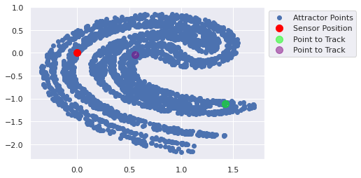
2.4. Measurement Problem
Now that we have a green point to track, suppose that we only have a measurement device at the origin which can measure the distance (like a RADAR device).
# Prior state estimate: \hat{x}^{-}
true_state = jnp.array([1.25, 0])


# Prior covariance: P^{-}
prior_covariance = 1/16 * jnp.eye(2)
prior_estimate = true_state + 1/4 * jax.random.normal(subkey, shape=(2,))
key, subkey = jax.random.split(key)

# Nonlinear Measurement 'h'
@jit
def measure(true_state):
    return jnp.linalg.norm(true_state)

# Measurement Covariance: r
measurement_covariance = jnp.array([1/4])

# Measurement: y = h(x) + eta
measurement = measure(true_state) + jnp.sqrt(measurement_covariance) * jax.random.normal(subkey)
key, subkey = jax.random.split(key)
First let us see how the system evolves.
def track_point(time_units, true_state, prior_estimate, prior_covariance, update_method, update_method_kwargs):
    """
    Given a starting (true) point, a prior estimate of the state, a prior covariance of the state, a
    """
    for time_unit in range(time_units):
        plot_ikeda_points([
             {'x':0,'y':0,'c':'red','label':'Sensor Position','s':100},
             {'x':true_state[0],'y':true_state[1],'c':'lime','label':'Point to Track','s':100, 'alpha':0.5},
             {'x':prior_estimate[..., 0],'y':prior_estimate[..., 1],'c':'purple','label':'Point to Track','s':100, 'alpha':0.5},
        ])
        plt.show()
        true_state = ikeda_update(true_state)
        print(prior_estimate)
        prior_estimate, prior_covariance = update_method(prior_estimate, prior_covariance, **update_method_kwargs)

track_point(time_units=10,
            true_state=jnp.array([1.25, 0]),
            prior_estimate=jnp.array([1.25, 0]), #+ jax.random.uniform(minval=-0.1, maxval=0.1, key=key, shape=(100,2)),
            prior_covariance=jnp.eye(3),
            update_method=lambda x_1, x_2, **x: (ikeda_update(x_1)+ 0.01, x_2),
            update_method_kwargs={})

[1.25 0. ]

[ 0.6024831 -1.0385966]

[-0.06979907 -0.03225724]

[ 0.98181725 -0.05320451]

[ 0.20815751 -0.3643704 ]

[1.3358982 0.20086011]

[ 1.0052788 -1.2058134]

[ 0.16977595 -1.1259253 ]

[0.10684864 0.4942605 ]
[ 0.5582348 -0.04507566]
2.5. Measurement
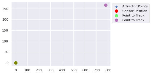
Now that we have a green point which we want to follow, we now construct a new estimate, a purple point,
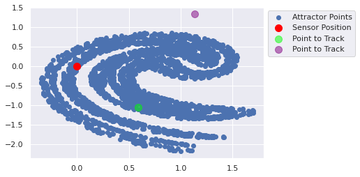
2.6. Bayesian Recursive Update
def bayesian_recursive_update(prior_estimate, prior_covariance, measurement, measurement_covariance, num_steps):
    state_estimate = prior_estimate
    covariance = ikeda_jacobian(prior_estimate) @ prior_covariance @ ikeda_jacobian(prior_estimate).T

    measurement = prior_estimate
    for _ in range(num_steps):
        measurement_jacobian = jax.grad(measure)(state_estimate)
        kalman_gain = covariance @ measurement_jacobian.T * (measurement_jacobian @ covariance @ measurement_jacobian.T + num_steps * measurement_covariance) ** (-1)
        state_estimate = state_estimate + kalman_gain * (measurement - measure(state_estimate))
        covariance = (jnp.eye(2) - kalman_gain @ measurement_jacobian) @ covariance
    print(state_estimate)
    return state_estimate, covariance

track_point(time_units=10,
            true_state=jnp.array([1.25, 0]),
            prior_estimate=jnp.array([1.24, 0]),# + jax.random.uniform(minval=-0.1, maxval=0.1, key=key, shape=(100,2)),
            prior_covariance=jnp.eye(2),
            update_method=bayesian_recursive_update,
            update_method_kwargs={'measurement':measure(jnp.array([1.25, 0])), 'measurement_covariance':measurement_covariance, 'num_steps':20})

[1.24 0. ][1.1314527 1.3454187]
[1.1314527 1.3454187]
[ 0.8926025  -0.91010994]

[ 0.8926025  -0.91010994]
[0.6987301  0.01448113]

[0.6987301  0.01448113]
[779.3692 267.2606]
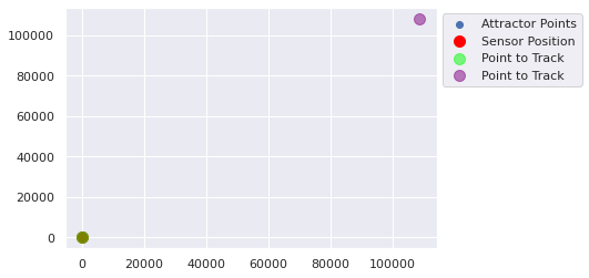
[779.3692 267.2606]
[108752.64 108246.95]
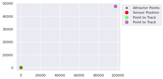
[108752.64 108246.95]
[97646.51  47751.188]
[97646.51  47751.188]
[nan nan]

[nan nan]
[nan nan]

[nan nan]
[nan nan]

[nan nan]
[nan nan]
2.7. Test
#key, subkey = jax.random.split(key)
#ensemble = jnp.array([1.25, 0]) + jax.random.uniform(minval=-0.5, maxval=0.5, key=key, shape=(100,2))
#ensemble.mean(axis=0)

jnp.linalg.inv(jnp.array([[2]]))


def func(x1, x2):
    pass

func(**{'x1':1, 'x2':2})